
How to Create a Column Chart in Google Sheets
Step-by-Step Guide to Creating a Column Chart
Creating a column chart in Google Sheets is a great way to visualize your data and make it easier to understand. With just a few simple steps, you can create a professional-looking chart that helps you to identify trends and patterns in your data. In this article, we will show you how to create a column chart in Google Sheets and provide you with some tips on how to customize it to suit your needs.
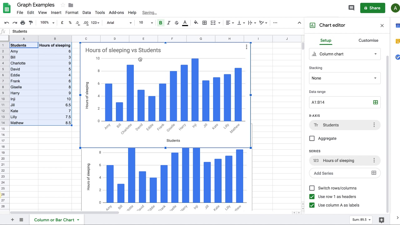
To create a column chart in Google Sheets, you need to start by selecting the data that you want to use for your chart. This can be a range of cells that contains the data that you want to visualize. Once you have selected your data, you can go to the 'Insert' menu and select 'Chart'. This will open up the chart editor, where you can choose the type of chart that you want to create. In this case, you will want to select 'Column chart' from the list of available options.
Customizing Your Column Chart
Once you have selected the column chart option, you can customize your chart by adding a title, labels, and other elements. You can also change the colors and fonts used in your chart to match your brand or personal style. To add a title to your chart, simply click on the 'Title' field and enter the text that you want to use. You can also add labels to your chart by clicking on the 'Labels' tab and selecting the type of label that you want to use.
Finally, you can customize your column chart even further by using the various options available in the chart editor. For example, you can change the axis labels, add gridlines, and modify the chart's layout. You can also use the 'Advanced edit' option to make more detailed changes to your chart, such as changing the font size and color. With these tips and tricks, you should be able to create a professional-looking column chart in Google Sheets that helps you to visualize your data and make informed decisions.